This post was inspired by the session “Managing many models with R” from Hadley Wickham. He reviews a few tidyverse principles, including nested data, functional programming, and how to tidy and visualize the output of models. The key takeaway for me was the latter point: how to fit multiple simple linear regression models across categories and summarize the models with visualizations.
I thoroughly enjoyed the session and it go me thinking how I could translate some of these principles and workflows to Power Query in Power BI.. I’ll cover how I took inspiration from the example in R and how I was able to replicate the workflow in Power BI.
The .pbix file I built can be found here.
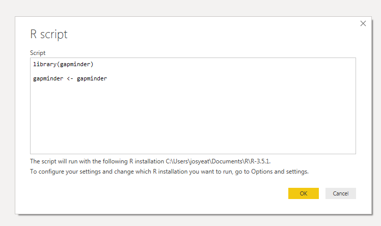
The data used in the example is from the gapminder package in R. I used the following R Script as a data source for my Power BI. I loaded the gapminder package and stored the data set in an object also named gapminder. For more on using R scripts as a data source, check out my previous post on the topic.
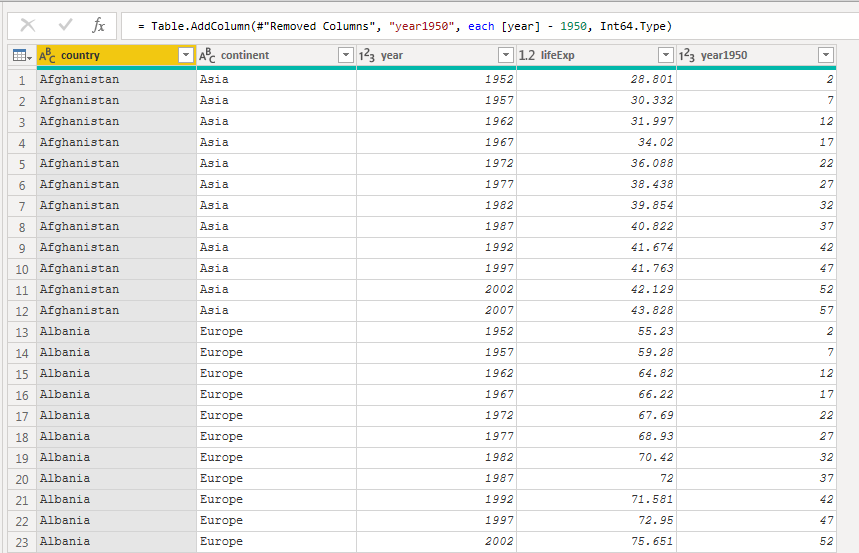
I created the initial query, Gapminder, by navigating to this object and expanding the results. I removed two columns and created a new one: year1950. This subtracts the value of 1950 from each year in the data set, calculating the number of years after 1950.
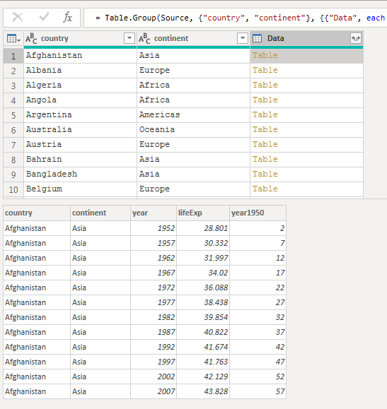
I referenced Gapminder to create a new query: Nested Gapminder. The goal of this query was to transform the data set to have one row for each country. This requires nesting, or aggregating, the other columns in the query.
In R, this can be achieved using group_by() and nest(). In Power BI, I used the group by functionality and selected the aggregation of All Rows. This differs slightly from the R as all of the columns in the data set are grouped instead of only the columns excluded from the aggregation.
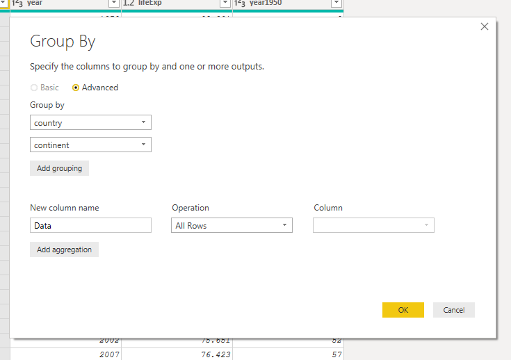
The grouping left the query with three columns:
- Country
- Continent
- Data – a complex column with a table in each row. The table contains the aggregated rows (year, life expectancy, year 1950) associated with the country.
The goal was to create a linear model for each country, using the nested data contained in the “data” column. In R, this can be achieved by creating a function to generate the linear model, then use map() to apply this function to each country.
In Power BI, I decided to build a model for one country, convert the transformation steps into a function, then create a new column in the query by invoking this custom function on each of the countries.
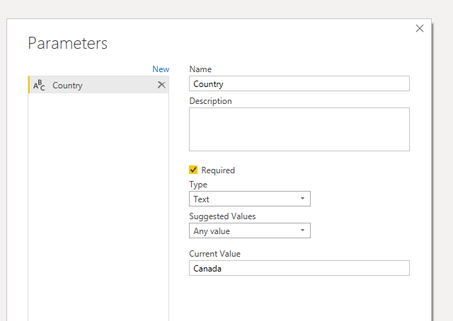
Before I started to build the logic to create the linear model, I knew that the function would need a parameter. Since I wanted to run the query on one country at a time, the parameter should contain the name of the country.
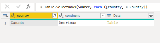
My first step was to filter the query so that the country column was equal to the value of the Country parameter.
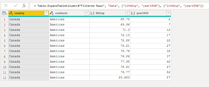
Now that the data was filtered down to one country, I expanded the data column to return all of the rows inside the table (that had been aggregated earlier).
This is when I started to create the linear model. But first, a quick aside..
A simple linear regression model can be expressed as the equation:
y = ax + b
This takes me back to math class in high school.. This equation models a data set by expressing the relationship between the x and y variables. These variables are two columns from the data set. Each observation, or row, from these two columns can be plotted visually on an x- and y-coordinate as a scatter plot. This can provide a basic understanding of the shape of the data set.
The goal of a simple linear model is to fit a line onto this plot to summarize the shape of the data using the equation above.
The “a” value is the slope of the fitted line (rise over run) and the “b” value is the intercept on the y-axis (when x is equal to zero).
In the gapminder example, the life expectancy column was assigned as the “y” variable, as it is the outcome that we are interested in predicting or understanding. The year1950 column was assigned as the “x” variable, as it is what we are using to try and measure the change in life expectancy.
The value of x (number of years from 1950) will always be known, so to generate a prediction of the y value (life expectancy) we need to calculate the slope of the line (how life expectancy is expected to change each year after 1950) and the y-intercept (expected life expectancy when x is zero, or when the year is 1950).
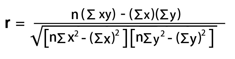
The values of a and b can be calculated using the following formulas:
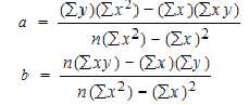
Which looks daunting, but is actually straightforward. To summarize, I needed to create or identify values for:
- x
- y
- x2
- y2
- xy
- n
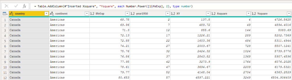
But we already have half of these values! We know x is the year1950 column. The lifeExp column is our y value. The n value is the number of rows.
This left three values to create. The xy column I created by adding a new column, multiplying lifeExp and year1950. The remaining two values I created by using the =Number.Power() function on the lifeExp and year1950 columns.
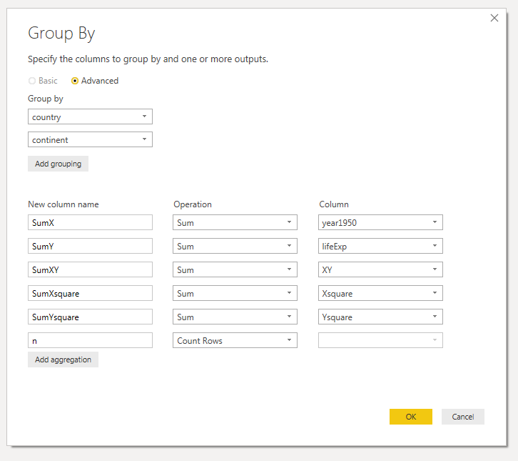
Now that all of the values have been created, I can create the aggregations using a Group By to:
- sum the values
- count the number of rows
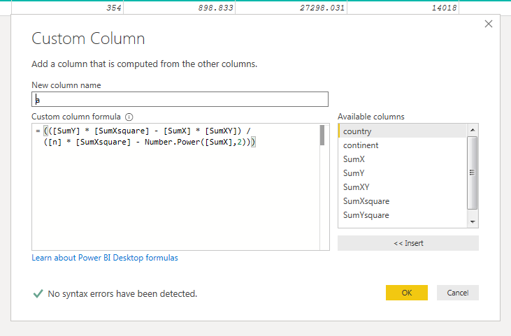
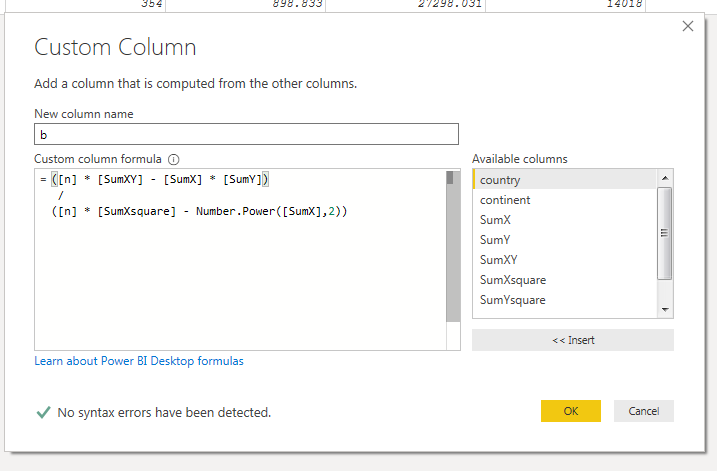
At this point, I had all of the values that I needed to plug into the two equations outlined above. I created both using a custom column.
Now that we have our model, we need to measure how well our model performs! One such measure of model performance is R2. This measures how much of the variability of the y variable, lifeExp, is captured by the x variable, year1950. Put another way, how much of the change in y is explained by the change in x.
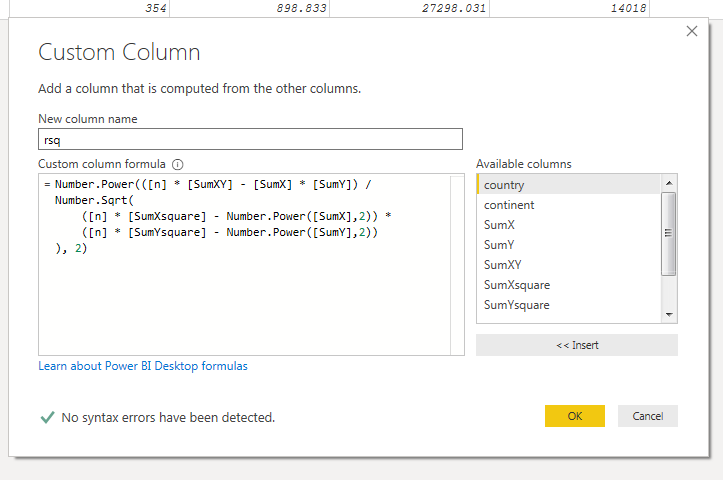
The formula to calculate R2 is:
Once again, I created a custom column and plugged in the values I had created earlier.
Now for every country, I had the slope of the fitted line, the y-intercept, and a measure of performance for the model. I removed all of the other columns, as I didn’t need them for my analysis.
At this point, I converted these transformation steps into a function. Then I created a new column on the original nested data set by invoking this function on each of the countries.
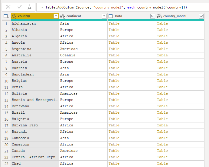
I expanded the new column to retrieve the three values I created with the function for each of the rows.
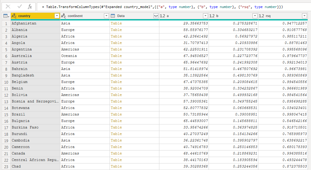
I closed and loaded the query and built two visuals. These visuals are the same as two built with the ggplot2 package in the “Managing many models with R” presentation.
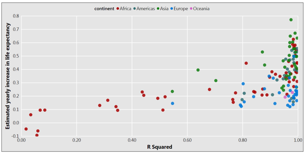
The first visual plots the slope of the line against the model performance using a scatter plot. Each observation in the visual is a country and the color corresponds to which continent the country belongs to.
It’s quick to see that the simple model performs quite well, with lots of countries having a large R Squared. Almost all of the countries with poor performance are from the continent of Africa.
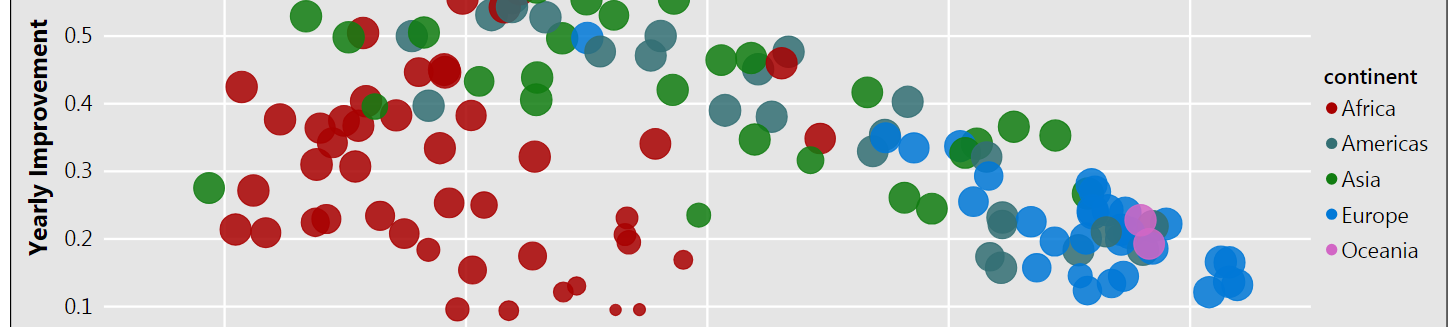
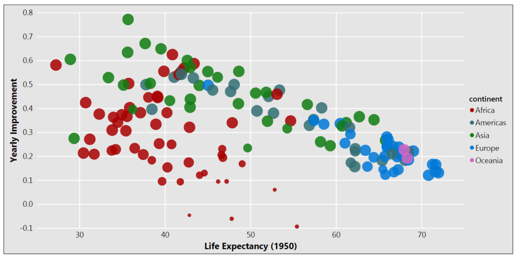
The second visual plots the slope of the model against the y-intercept. The size of the observation is based on the model performance.
Once again, it’s quick to interpret that countries from Europe and Oceania had a higher life expectancy in 1950 and subsequently have had a more modest annual increase. Countries from other parts of the world started out with a lower life expectancy, but have seen a higher annual increase in the years since.
I was pleased with the results of transferring tidy principles to Power BI and fitting multiple linear regressions models on the data set.
You are the one. Great Job.